 by a string of
 s.
We represent a sequence of
s.
We represent a sequence of
 natural numbers
 by a string of the form
 where
there are
where
there are

 s
between the
s
between the
 and
and

 We will use the notation
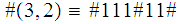
 to represent this string. For example,
We represent a natural number
by a string of
s.
We represent a sequence of
natural numbers
by a string of the form
where
there are
s
between the
and
We will use the notation
to represent this string. For example,
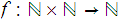
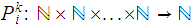
A function
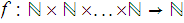 ,of
,of
 variables, is called Turing Computable if there exists a
Turing Machine
variables, is called Turing Computable if there exists a
Turing Machine

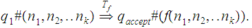
such that for all
 we have the derivation
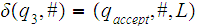
Example: Suppose

then
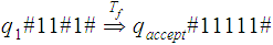
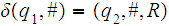
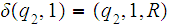
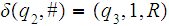
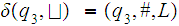
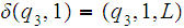
1. The successor function
 is Turing Computable:
Assuming that the input tape is as above, one can easily define


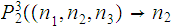
2. The projection functions
 are Turing Computable.
Homework: Due November 17 :
Show that
 is Turing Computable.
3. The set of Turing Computable functions is closed under composition.
For simplicity we consider the case of two functions of a single variable.
Assume
 and
and
 are Turing Computable by Turing Machines

 and
and
 We
need to produce a Turing Machine
We
need to produce a Turing Machine
 that computes
 .
.
By selecting alternative members, we can assume that the set of states of

 and
and
 are
disjoint. We let
.
are
disjoint. We let
. denote a generic state of
 and
and
 denote a generic state of
 .
.
With some addition bookkeeping the work is to construct an appropriate
transition function. We start with the union of the two sets of 5-tuples.
 Next replace all occurrences of
 with
with
 . Finally, replace all occurrences of
 with
with
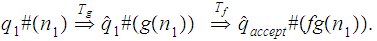
 Derivations have the form
A function is recursive iff it Turing Computable. With appropriate modifications of the relevant definitions, this also holds for partial recursive functions.