The first step is to represent the problem mathematically. In this case, we will have two variables, x and y, where x represents the number of Fruit Basket A to make and y represents the number of Fruit Basket B to make. We know that each Fruit Basket A sells for $8 and each Fruit Basket B sells for $12, but in order to know how much profit we will make, we must compute the costs of each basket. Basket A contains 3 apples @ $ .30, 4 oranges @ $ .20 and I melon @ $1.20, so it costs $2.90 to make up the basket (if we assume the actual basket is free). Hence, the net profit from Basket A is $5.10. Using a similar method, we can find that the net profit from Basket B is $7.80. Hence, our objective is to:
maximize 5.10 x + 7.80 y
However, there are constraints dictating the availability of fruits which must be met. Using the quantities above, they are
Apples: 3x + 4y < 160
Oranges: 4x + 3y < 180
Melons: 1x + 2y < 60
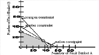
Conceptually, the algorithm for solving this problem looks at possible values for x and y and selects the one that maximizes our objective. Consider the graph below.

The algorithm “knows” to look for the feasible combinations of the two types of Fruit Baskets, as shaded in the graph. Further, it “knows” that the best combination is going to be one of the four “extreme” or corner points highlighted above. The algorithm evaluates an extreme point with regard to the objective (5.10x + 7.80y). It then looks at the adjacent corners to determine if one of them give a better solution. If so, the algorithm moves to that new point and begins again. In essence, the algorithm moves from corner to corner, always improving the value of the objective. With large problems, the process is important because one can have many variables and many constraints resulting in millions of corner points. Since the algorithm follows a systematic approach to improvement, it ends up checking only a small percentage of the possible points. In this case, it is the combination of 36 Fruit Baskets of Type A and 12 Fruit Baskets of Type B, giving a profit of $277.20 to the MIS Club.