
Do we focus on the first question that comes up, or is there a way to check out the best questions to ask? This issue is central to education, as well as e.g. to policy discussions of all sorts.
In particular, how might we best make our choice of concepts informed to the data at hand? Put another way, what does the practical discipline of theory-selection have to say?
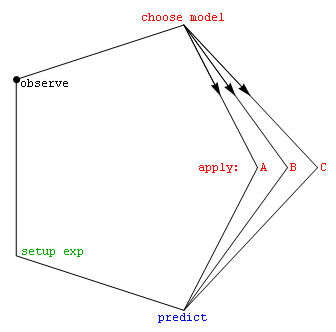
We explore here the possiblity that ad-hoc tables of observations versus models, designed to catalyze a narrative about how various idea-sets are more or less surprised by stuff seen in the world around, can help us do a better job at combining different points of view constructively...
The basic idea is simple: Recognize that we live in a world with new data continually arriving, to help us avoid the temptation to skip the job of assessing our concepts, models, and actions in light of that datastream. This also lets us cast old approaches (e.g. via the tables discussed below) in light of the observations that their developers had to work with. Rather than locking ourselves into arguments about the true/false nature of old assertions (based on different and possibly less information than we have now), this might help us gain from the strengths and weaknesses of all approaches, old and new, as we look toward unfolding challenges, individually and collectively, in the days ahead.
The science of Bayesian-inference applied to model-selection may eventually offer a quantitative way to assess such new approaches. That's because log-probability based Kullback-Leibler divergence, or the extent to which a candidate model is surprised by emerging insights, formally considers both goodness of fit (prediction quality) and algorithmic simplicity (Occam's razor). This strategy lies at the heart of independent approaches to quantitative model-selection in both the physical[1] and the life[2] sciences.

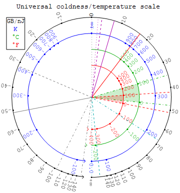
In this technical draft note for physics teachers we review the basis for quantitative Bayesian model-selection, and then qualitatively review old news e.g. that: (i) proper velocity and acceleration are useful over a wider range of conditions than their coordinate siblings; (ii) uncertainty, and uncertainty slopes like coldness 1/kT, provide insight into a wider range of thermal behaviors than does T alone; and (iii) entropy has deep roots in Bayesian inference, the correlation-measure KL-divergence encountered self-referentially above, and simple measures for effective freedom of choice. A set of ten potentially-useful appendices is then provided for those looking to explore specific aspects of these connections with their class.
This web-page is meant to be less discipline-specific, and explore an alternate but robust way for folks to explore on their own terms the way that our evolving ideas connect to our unfolding observations about the world around them.
The quantitative science of model-selection has made concordant but independent strides in both the physical and life sciences toward assessing the ability of models to describe observations. Recent developments in particular assess both goodness-of-fit and (via an "Occam-factor") simplicity of presumption by using a log[1/probability] measure that Myron Tribus (we think) first referred to as "surprisal". Surprisal is measured using information units (like bits), and lies behind our understanding of thermodynamics as well as our methods for tracking genetic-relatedness and compressing-data, to mention only a few of its current applications.

Can the vernacular concept of surprise similarly capture the effectiveness of scientific idea-sets to predict and describe new observations? This page is set up to explore the possiblity that, at least qualitatively, the tabulation of surprises might help bring the discussion of competing idea-sets into closer contact with the observations that inspired them.
These might be good places to post talk notes for moderated commentary.

Some possible issues that might be fun to think about in this context are listed in the sections below.
What would your table of idea-sets and phenomenological surprises look like for these topics?
For what other topics might you be inclined to put together similar tables?
As a quantitative example to start off with, consider a set of electrostatic force measurements (with measurement errors of ±0.2 force units) as a function of radial distance, like for example the following {separation-distance, force} pairs: {{0.8, 1.64204}, {0.9, 0.891087}, {1., 1.0413}, {1.1, 0.898058}, {1.2, 0.917022}, {1.3, 0.762478}, {1.4, 0.465493}, {1.5, 0.571502}, {1.6, 0.601989}, {1.7, 0.431092}, {1.8, 0.256245}, {1.9, 0.331824}, {2., -0.00813074}}.
Let's compare the extent (in bits or surprisal) to which an unknown power-law, and a one-over-r-squared power law, are surprised by this data. The maximum-likelihood parameter-estimates for the a/rb model are {a -> 1.01717, b -> 1.76984} while the maximum-likelihood parameter-estimate for the a/r2 model is {a -> 1.01833}.
If we choose parameter-priors using Akaike Information Criterion, the cross-entropy surprisals (in bits) of each model at this particular data-set are:
| \Models observations | unknown power a/rb | action at distance a/r2 |
|---|---|---|
| dataset 1 | 9.61 bits | 8.01 bits |
Over a sample of 10,000 such datasets, the average surprisal at the data by the unknown power-law is about 1.31 bits larger than the suprisal of the generating one-over-r-squared power law, in spite of the fact that the extra free-parameter in the unknown power-law always generates a closer fit to the data.
Here's a subjective tabulation of "surprise" exclamation-marks that might be attributed to mostly 19th century idea-sets (columns in the table) associated with the everyday properties of electricity and magnetism, when those idea-sets encounter observations of various phenomena (rows in the table) which might have been unexpected at first even if on reflection said idea-sets could fit them into their picture. If the screen you're reading this on is indicative, the awareness provided by these models continues to serve us well even into the 21st century.
| \Models nature's surprises | Tempermental deities | Action at a distance models | Faraday's lines of force in space | Clerk Maxwell's flux equations |
|---|---|---|---|---|
| lightning | ||||
| electrostatic 1/r2 | ! | |||
| magnetic filing alignment | ! | ! | ||
| charging-capacitor gap B-field | ! | ! | ! | |
| electromagnetic radiation | ! | ! | ! | |
| the flat-space metric equation | ! | ! | ! |
Although any of the natural behaviors listed in the left column might be explained after the fact by tempermental deities, there was for example no deity-model which predicted (in advance) that electrostatic repulsion would fall off inversely as separation r squared and not as separation to some other power. The exponent of r was therefore a fit-parameter in the deity models not needed in the action-at-a-distance models, which (like Newtonian gravity) behaved in this way because of the 3 spatial-dimensions in which they were embedded. In that sense the deity-model either predicted with less precision, or was able to predict accurately only after lots of data had been obtained to empirically-determine the exponent to be approximately 2.
Below find a more technical tabulation that (having been long involved with electron phase-contrast imaging of atomic lattices) I might attribute to various idea-sets or paradigms for describing atoms and their constituents.
| \Models nature's surprises | Particle/Wave Dichotomy | Bohr-Like Hybridizations | Momentum's link to spatial-frequency | Feynman's view: Explore all paths |
|---|---|---|---|---|
| atom levels are quantized | ! | |||
| particle-beams diffract | ! | ! | ||
| single-particles self-interfere | ! | ! | ! | |
| mapping deBroglie phase-shifts across single electrons | ! | ! | ! |
The last row in this table is inspired by the fact that high-resolution transmission-electron-microscope images of thin specimens on size-scales larger than the operating point-resolution can be interpreted as quantitative maps of exit-surface deBroglie phase-shift across the coherence-width of individual electrons. This is an interesting fact about a process that, regardless, is becoming increasingly useful in everyday detective-work on solids at the nano-scale.

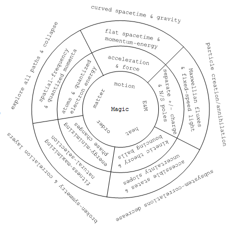
As discussed with examples in the technical note, this table might cover both the transition from pre-Galilean impetus theories, through Newtonian insights about everyday motion, to Einstein's electromagnetically-informed recognition of Minkowski's metric-equation path to understanding accelerated motion at any speed plus spacetime curved by gravity. A similar transition from Lorentz to metric-equation views of motion at any speed is happening gradually in textbooks today. What else?
As likewise discussed in that technical note, this table might include things like the move from phlogiston/caloric theories, through the recognition that heat is a form of disordered energy to which statistical inference applies, and through the entropy-first approaches which gained a foothold in the 19th century with help from Maxwell, Boltzmann plus Gibbs and have pretty much taken over senior-undergrad physics texts (with Tom Moore's intro-physics text being one of the first to take that path). The 20th-century correlation-first strategy, which brings statistical physics back into contact with the broader application areas of statistical inference, is finding major applications e.g. in data compression and clade analysis, but is not yet widely discussed in context of its promise for helping us with modern cross-disciplinary challenges like community health. The stretch may be less than you imagine, as general systems theory already has a track record of helping toward such ends.
This table of surprises will likely involve geocentrism and Ptolemaic epicycles, Brahe and Galileo's observations & heliocentric simplifications, Kepler and Newton's insights about orbital mechanics; plus more recent planetary-mission and extra-solar planet data along with laboratory observation of: lunar/cometary sample returns, stratosphere-collected interplanetary dust, and pre-solar stardust from meteorites.
One might also include in these surprises the extra-galactic observation of red-shifts, the 3K background, fluctuations possibly linked to inflation, effects of apparently-unseen mass, accelerated expansion, etc. These observations for the most part impact energy and length scales which, like details of the turtle on whose back the universe rests, are somewhat removed from the datastreams that we need to process in everyday life. Hence utility with data has historically taken a backseat to aesthetic factors in its impact on the model-consensus in these areas, making it all the more important in science classes to cover observations first.
What else?
This table will likely involve observations of volcanism and rock vibrations, plus models of planet formation and continental drift. What else?
This table might involve observations of weather's short-term unpredictability, as well as ice-core records (and models) of climate evolution. What else?
What observations called attention here to the ideas of species-formation by natural selection, trait inheritance and adaptation via the evolution of molecular codes, plus regulated gene-expression and epi-genetics? What else would you consider in putting together a table on this subject?
This table might involve e.g. Lorenz-style observations of behavior-redirection, behaviors correlated with gene-pool interests, insights into the co-evolution of genes and culture, more general mathematical models for the evolution of cooperation ala Nowak, and what else?
| \Models nature's surprises | chip off old block | behavior re-direction | code-pool natural-selection | evolving task layer-multiplicity |
|---|---|---|---|---|
| smiles & pair-bonding as aggression redirected[4] | ! | |||
| preferential treatment for one's own kids | ! | ! | ||
| gene-pool selection behind insect eusociality[5] | ! | ! | ||
| xenophobia about unfamiliar practices | ! | ! | ||
| humor[6] as a reward for model-rethinking | ! | ! | ||
| special-skills correlated with personality-flaws | ! | ! | ! | |
| natural tension between hierarchy & science | ! | ! | ! |
This table might involve data and models on subconscious brain-module operation, as well as its effect on the conscious gestalt, plus more recent data on brain physiology and models of brain function. What else?
This table might include observation of dietary requirements and the effects of exercise, concepts of carbon/water and caloric intake/output. What else?
This table might involve for example the surprise at market-share losses in the decade after Swiss mechanical watch-makers let Japanese & US companies offer the first new electronic quartz-watch types, even though prototypes were first made in 1967 by Swiss Centre Electronique Horloger (CEH) researchers in Neuchâtel. What other idea-sets have played a role here?
| \Models nature's surprises | self-slowing pocket-watches | mechanical wristwatch | electronic wristwatch | wireless wristcoms |
|---|---|---|---|---|
| balance wheel harmonic oscillation | ! | |||
| piezo-electric fork oscillation | ! | ! | ||
| electronic displays | ! | ! | ||
| wireless communications | ! | ! | ! | |
| voice/gesture input/output | ! | ! | ! |
This table might cover military and economic competition between governmental systems through various ages of evolving population and technology, plus the role of family, politics, culture and science in these various approaches. What else?
This table might examine the evolution of gender and cultural role-specialization, plus its diversity, as a function e.g. of both information flow, and the rate at which a community manages to consume available work. What else?
Clearly a tabulation of approaches which eventually led to these surprise-tabulations here is worthwhile, although it may take a while to pull this one into focus. Frequentist statistics might play one role here, and what else?

In that technical note, Gregory's marginalization and his Occam factor involve specific decisions about fit-parameter prior-probability i.e. the ΔAα ∀ α ∈ {1,K}. On the other hand Akaike Information Criterion (AIC) suggests that one simply use ln[1/ΩM] = NK/(N-K-1) ≈ K when N>>K. This is a simple penalty (for large N) of one "nat" of surprisal for each added fit-parameter, although in the AIC literature this simple result is obscured by the choice of non-traditional information-units (in effect Akaike uses logs to the base Sqrt[e]).
Taking that suggestion is equivalent to using a uniform-prior range for each parameter e.g. equal to ΔAα = Sqrt[2πVα]eN/(N-K-1) ∀ α ∈ {1,K}, where N is the number of data-points, K is the number of fit-parameters, and Vα is the eigenvalue of the K×K parameter covariance-matrix V associated with fit-parameter Aα. When one doesn't have prior information on fit-parameter ranges, therefore, this is an elegant choice that allows one to parsimoniously apply two independently-derived Bayesian model-selection strategies toward a shared result.